Time in MAQL (Time Macros & Time Transformation in GoodData.CN)
Version Compatibility Notice
The content of this article is valid for the version of GoodData that was current as of 2 August 2021. Features or behavior in newer versions may differ.
Time Dimension in GoodData.CN
Time is a useful entity for data analysis and is one of the most frequently used dimensions on dashboards. Sometimes, you may want to compare the numbers in different periods. In this article, we will focus on how to use Time Macro syntax to segment the data in various date/time dimensions in GoodData.CN.
Time Macros
Time Macros in MAQL allow you to reference the metrics relative to the present. You may use THIS, PREVIOUS, NEXT to segment the date granularities relative to the present day. It is very powerful when comparing the numbers between the present and the same day of a different period. The available date granularities include day, week, month, quarter, year, day of the week, day of the month, month of the year, etc. Some useful functionalities may include: How many orders were made last Monday? Or how much revenue was made in August of the previous year?
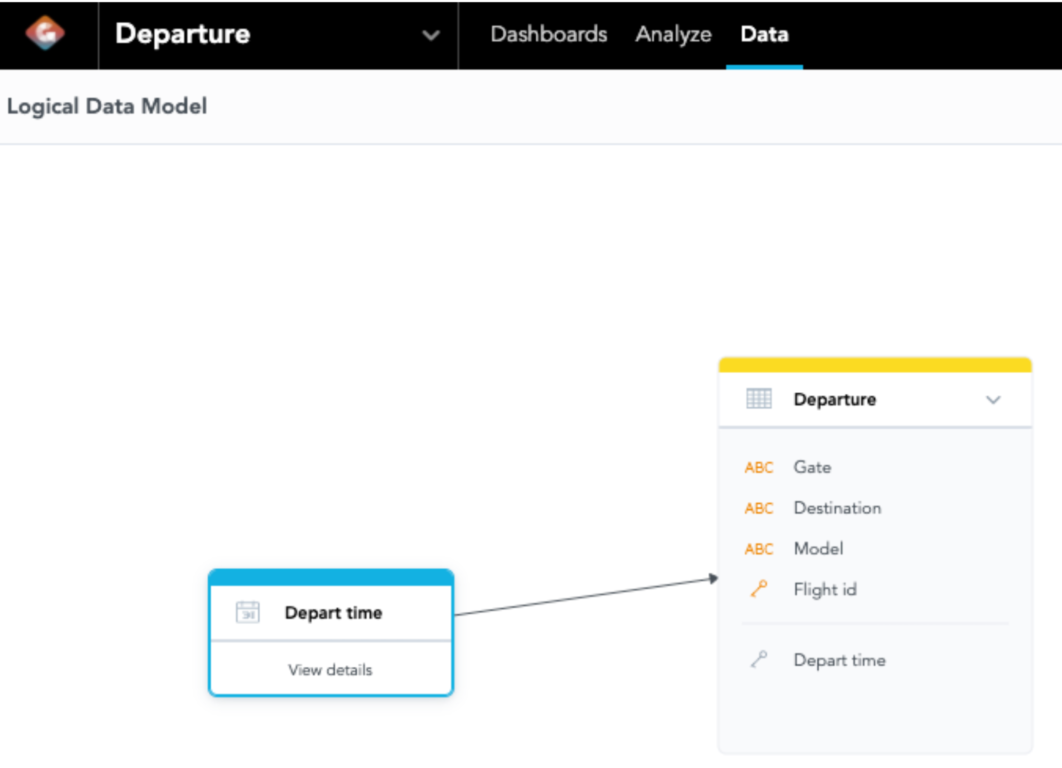
To achieve our goal, it is easier to demonstrate with an example: Let’s pretend we are conducting an analysis of the departure flights in an airport. Our dataset has Flight ID, departure time with date and time, destination, gate, and the aircraft model used in the table Departure Time. The following diagrams show the Logical Data Model (LDM) and its metadata:
Diagram 1: LDM of Departure
| Type | ID | Column Name in LDM |
|---|---|---|
| Attribute | departure.gate | Gate |
| Attribute | departure.destination | Destination |
| Attribute | departure.model | Model |
| Attribute | departure.flight_id | Flight ID |
| Date | depart_time. |
Depart time |
Table 1: Metadata of the Workspace
In this dataset, we have the records of the flights with their flight number, departure date and time, gate, and destination in IATA code (Example: LAX for Los Angeles International Airport). Let’s say I want to know how many flights are departing from today. We can use the following syntax for the number of flights departed today:
Syntax 1:
SELECT count({attribute/departure.flight_id})
WHERE {label/depart_time.day} = THIS(DAY)
The label “depart_time.day” in the where clause segments the data by day and uses “THIS(day)” to reference the query to only focus on today. You may change the date granularities by replacing the day with different granularities. For example, if you want the number of flights departed in the previous week, you may change the syntax to:
Syntax 2:
SELECT count({attribute/departure.flight_id})
WHERE {label/depart_time.week} = PREVIOUS(WEEK)
Likewise, you may use “Next” to replace “Previous” or “This” if you would like to compare data with the future date (Perhaps comparing today’s number with the number of scheduled flights in our case). Here is the date granularity you may use in GoodData.CN and its ID:
| Type | ID | Granularity |
|---|---|---|
| Date | Day | |
| Date | Month | |
| Date | Quarter | |
| Date | Year | |
| Date | Week | |
| Date | Week of Year | |
| Date | Month of Year | |
| Date | Quarter of Year | |
| Date | Day of Month | |
| Date | Day of Week | |
| Date | Day of Year |
Table 2: List of Date Granularity Available in GoodData.CN
You may add an integer as a parameter into the previous keyword, like PREVIOUS(week, 2), to indicate the magnitude of the period to be segmented. Currently, GoodData.CN does not support any granularity below day for Time Macros, including hour and minute.
Time Macro is very powerful when you compare metrics between two different periods of time. If you are interested in comparing the difference between the number of flights last week and today, we can use the following MAQL query:
Syntax 3:
Select (
    (Select count({attribute/departure.flight_id})
    WHERE {label/depart_time.week} = THIS(week))
    - (Select count({attribute/departure.flight_id})
    WHERE {label/depart_time.week} = PREVIOUS(week))
)
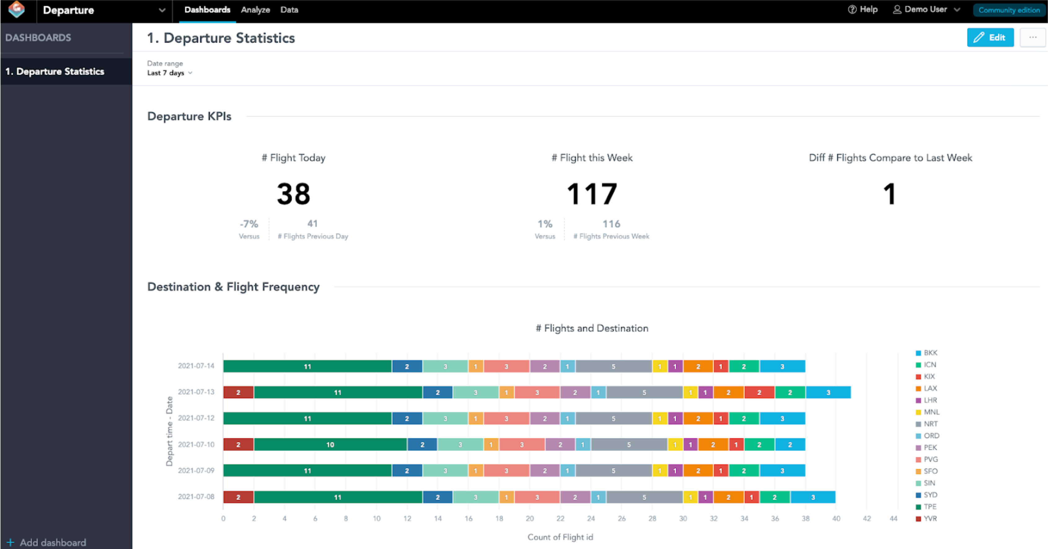
Once we have those metrics defined we can create KPI headlines or other visualizations in Analytical Designer and end up with a dashboard that looks like this:
Diagram 2: Dashboard for Departure Statistics
Time Transformation
Time transformation in MAQL allows the flexibility to calculate the metric when you have an additional time granularity in the visualization. The syntax of time transformation is FOR Next, FOR NextPeriod, FOR Previous, and FOR PreviousPeriod.
Both FOR Next and FOR Previous allow you to shift the time frame forward and backward relative to the time granularity. For example, I need a metric to count how many flights are departing to Taipei (TPE) in the next hour, you may define this metric as:
Syntax 4:
SELECT count({attribute/departure.flight_id})
FOR Next({label/depart_time.hour})
WHERE {label/departure.destination} = "TPE"
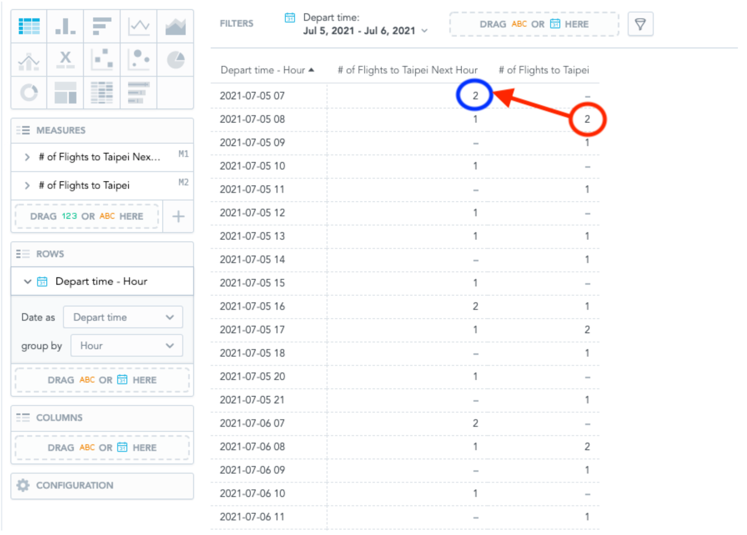
Diagram 3: Count the number of flights to Taipei
If we use this metric on a table like Diagram 3, we can see that it will count the number of flights departing to Taipei in the next hour. We know that there are 2 flights departing to Taipei in the 8 AM hour slot on 07/05. Therefore, it is reflected on the first column in the 7 AM hour slot on 07/05 after we have applied the metric with Syntax 4.
You may also add an integer as a parameter into the next keyword, like Next({label/depart_time.hour}, 2), to indicate counting the number of flights in the next 2 hours ahead. Note that the Where clause should be placed after the For Next function.
The difference between FOR Next and FOR NextPeriod is that FOR Next sets the values at a fixed time frame transformation while FOR NextPeriod sets the values at a flexible time frame. Let’s continue the discussion using an example. For example, we have two flights departing to Toronto (YYZ) on 07/23 and 07/24:
Syntax 5:
SELECT {metric/num_flight_yyz}
FOR Next({label/depart_time.week})
Syntax 6:
SELECT {metric/num_flight_yyz}
FOR NextPeriod({label/depart_time.week})
Note: Metric num_flight_yyz is a metric counting the number of flights departing to Toronto (YYZ).
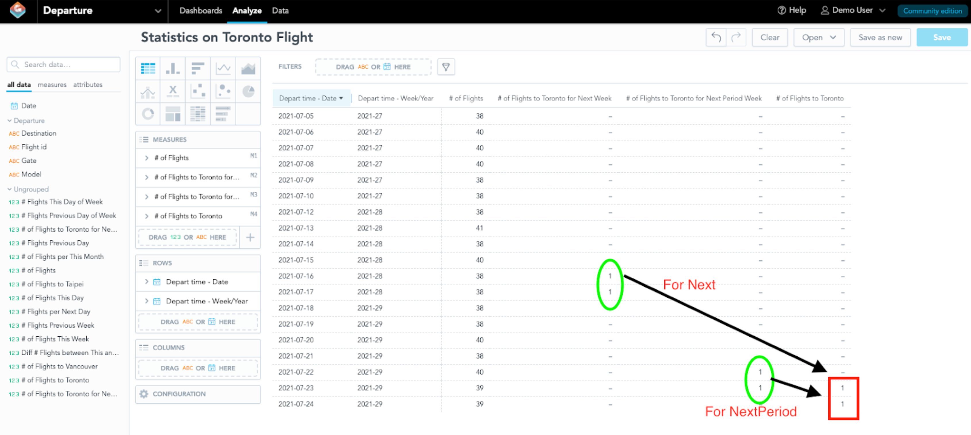
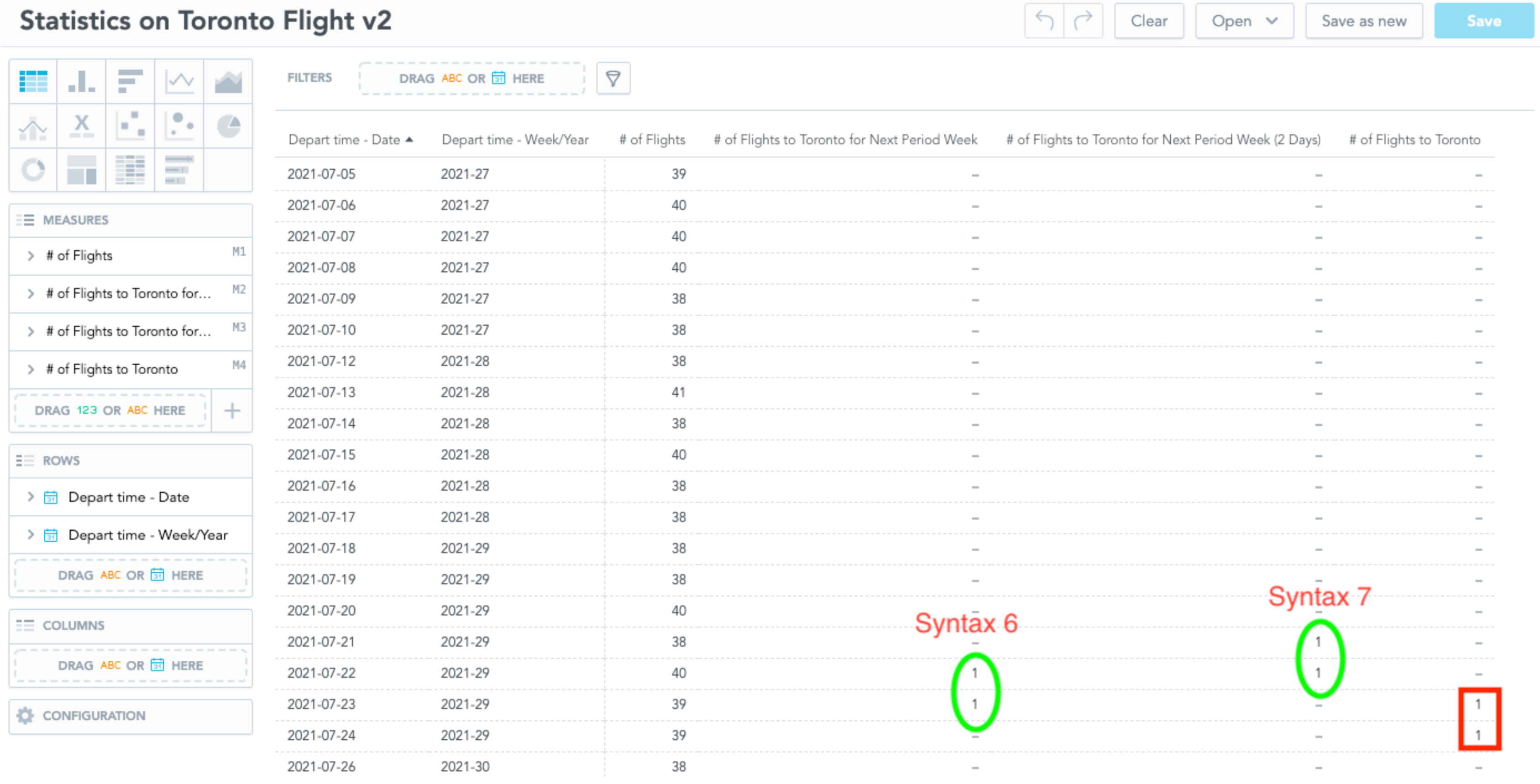
If we have plotted those metrics into a table along with the number of flights to Toronto and slides by day and week of the year, we would have a table like this:
Diagram 4: Statistics on Toronto Flight
“For Next” only looks at a fixed time frame in the metric. In our example, the metric defined with syntax only populates on 07/16 and 07/17 because there are flights departing to Toronto exactly in a week. “For NextPeriod” automatically takes the lower granularity available in the insight, even though the metric was set to week, the “NextPeriod” dynamically modifies the values to match the lower granularity present in the insight (In our example, it becomes the next day).
You may add another parameter into “For NextPeriod”, like Syntax 6 in the following:
Syntax 7:
SELECT {metric/num_flight_yyz}
FOR NextPeriod({label/depart_time.week}, 2)
The “2” in the “Next()” or “NextPeriod()” function indicates the magnitude of the period to show.
“Next(week, 2) will show the values available in exactly 2 weeks or 14 days after, whereas NextPeriod(week, 2) in our example above will take the lower granularity in the insight and show the values available in 2 days later. Syntax 7 will change the results to be counted on 07/21 and 07/22, like Diagram 5:
Diagram 5: Difference between Syntax 6 and Syntax 7
For Next and For NextPeriod differs between whether you would like the flexibility of the lower granularity if an extra granularity is segmented in an insight. One thing to note is if you leave the second magnitude parameter blank, it will default to “1”.
(Optional) Comparing between Day of Week
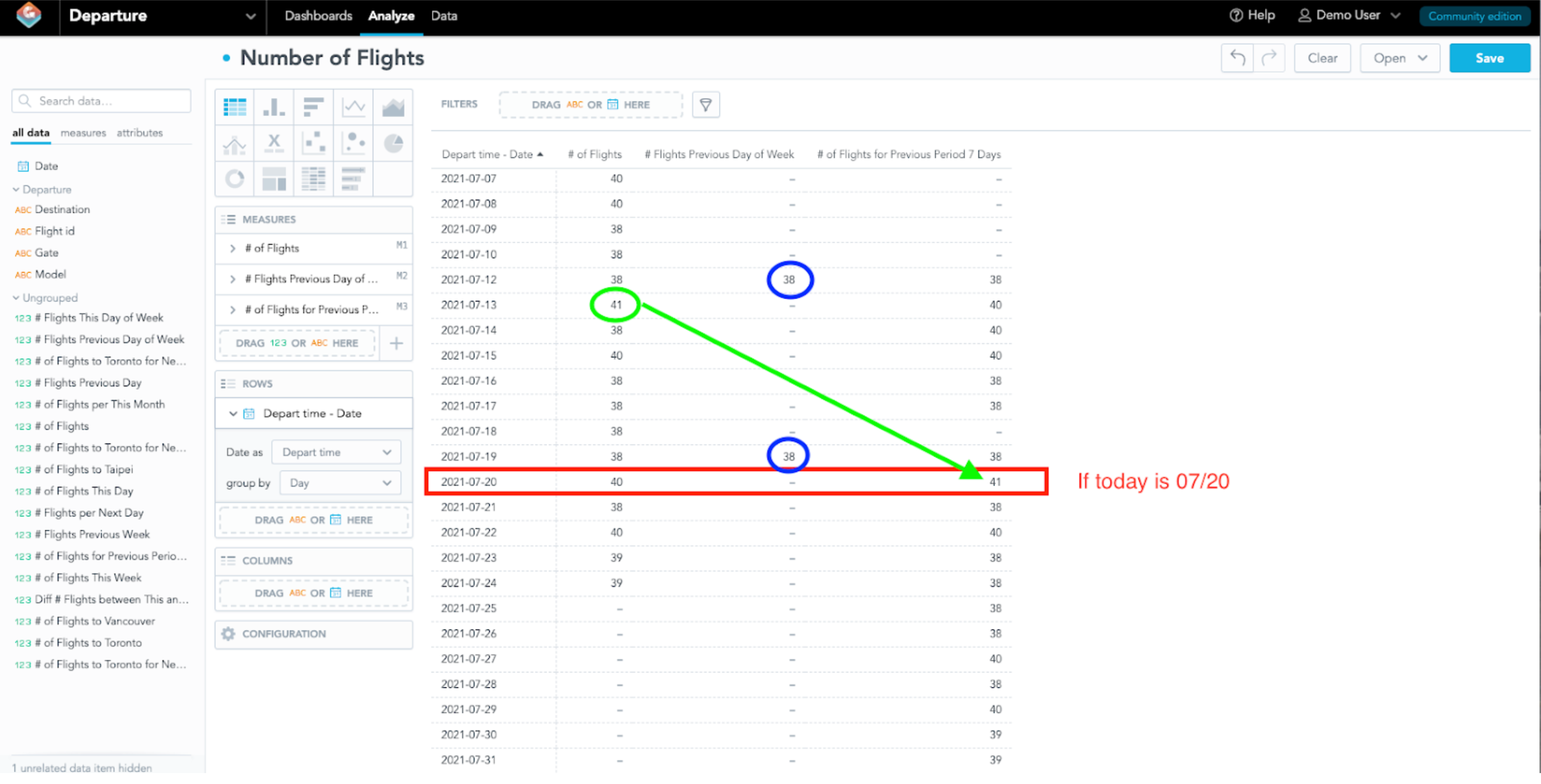
One confusion of using Time Macro is when the metric is defined with the day of the week. For example, if you define the metric with the following syntax and today is Tuesday 07/20:
Syntax 8:
SELECT count({attribute/departure.flight_id})
WHERE {label/depart_time.day} = PREVIOUS(dayOfWeek)
Syntax 7 counts the number of flights on the previous day of Tuesday (Which is Monday). The table will show the number of flights on Monday on every Monday entry. If you would like to show the number of flights on the previous Tuesday, you should define the following:
Syntax 9:
SELECT count({attribute/departure.flight_id})
FOR PREVIOUS(dayOfWeek, 7)
Diagram 6: Comparing Day of Week
