Hypothesis Testing - One Sample T-Tests and Z-Tests

This article describes how to use MAQL to build probability distributions and use them to perform hypothesis tests.

Background

Is an observed change in averages statistically significant? Suppose a company’s marketing team is monitoring daily Facebook Impressions and wants to know if the current month’s results are different from the historical results, perhaps due to an advertising campaign. Such analysis is a perfect candidate for hypothesis testing or significance testing.

The first step of hypothesis testing is to convert the research question into null and alternative hypotheses:

• The null hypothesis (H0) is a claim of “no difference.”
• The opposing hypothesis is the alternative hypothesis (H1). The alternative hypothesis is a claim of “a difference in the population.” It is the hypothesis the researcher often hopes to prove.

For our example company, suppose that the average Facebook impressions are 1000 per day before the campaign. The company believes that, owing to the ad campaign, the population now has higher average Facebook impressions. This means:

• (H0): μ = 1000
• (H1): μ > 1000

Next, we calculate the test statistic, which compares the observed sample mean to an expected population mean (in our example, this value is 1000).

The test statistic is then converted to a p-value, which tells us whether the result is significant or not. Small p-values provide evidence against the null hypothesis, as they indicate that the observed data are unlikely when the null hypothesis is true.

Here are the conventions the company uses:

• When p-value > .10 → the observed difference is “not significant”
• When p-value ≤ .10 → the observed difference is “marginally significant”
• When p-value ≤ .05 → the observed difference is “significant”
• When p-value ≤ .01 → the observed difference is “highly significant”

P-values depend on the direction of the hypothesis (left, right, or two-tailed):

• Right-Tailed: If you expected the ad campaign month to have more Facebook impressions than usual, your result is significant if the significance level is the 1 - p-value <=0.05, which is the same as p-value >= 0.95.
• Left-Tailed: If you expected the ad campaign month to have fewer Facebook impressions than usual, your result is significant if p-value is <=0.05
• Two-Tailed: If you don’t know whether the ad campaign month would have more or fewer Facebook impressions than usual, your result is significant if p-value is higher than 0.975 or lower than 0.025.

Calculating p-value

The first step is to upload a table of t-distribution values (cumulative left tail student distribution), which you can find in any statistical textbook. A sample CSV file is attached to this page:

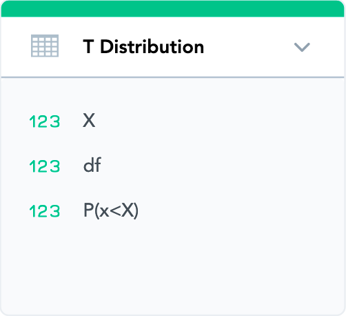
The example table has 3 columns:

• X: This is the lookup for the test statistic value from our sample.
• df: Lookup for Degrees of Freedom, which is equal to n-1 where n is number of records in our sample.
• P(x<X): p-value.

We’ll create a fact dataset in our LDM as shown below:

Note that the three columns are stored as facts.

After the values have been uploaded to the project, we can use the following metrics to calculate the p-value:

Pre-Campaign Avg (FB Impressions)

SELECT AVG(FB Impressions) BY ALL OTHER WHERE Month/Year(Activity Date) <> THIS

Here, we are calculating the average of FB impressions before the campaign. This value is known in layman’s terms as the ’long run average.’ We are treating it as the ‘population mean’ (μ₀) in this example.

Post-Campaign Avg (FB Impressions)

SELECT AVG(FB Impressions) BY ALL OTHER WHERE Month/Year(Activity Date) = THIS

This is our sample mean.

Post-Campaign StdDev (FB Impressions)

SELECT STDEV(FB Impressions) BY ALL OTHER WHERE Month/Year(Activity Date) = THIS

This is the standard deviation of our sample during the ad campaign month.

Test Statistic

SELECT ((Post-Campaign Avg(FB Imp) - Pre-Campaign Avg(FB Imp)) / (Post-Campaign STDEV(FB Imp) * (SELECT SQRT(n)))) BY ALL OTHER

The test statistic is defined as:

where:

• X̄ is the sample mean
• (μ0) is the population mean
• s is the sample standard deviation
• n is the number of records in the sample. In our example, n would be 30 or 31. We could always use the COUNT function in other cases.

X for p-value

SELECT (SELECT CASE WHEN Test Statistic < -10 THEN -10, WHEN Test Statistic > 10 THEN 10 ELSE ROUND(Test Statistic, 2) END) BY ALL OTHER

We’ve used ROUND because this metric will be used to look up the p-value in our distribution table where all the X values are rounded to 2 decimal points.

DF for p-value

SELECT (SELECT CASE WHEN n - 1 > 200 THEN 1000, WHEN n - 1 > 90 THEN 120, WHEN n - 1 > 45 THEN 60, WHEN n - 1 > 30 THEN 30 ELSE n - 1 END) BY ALL OTHER

Since we are looking at the current month in our example, n will be 30 or 31. This calculation will automatically switch from t-test to z-test if the number of records is higher than 150, which is explained in the last paragraph.

p-value

SELECT (SELECT SUM(P(x<X) WHERE df = df for p-value and X = X for p-value) BY ALL OTHER

This metric provides the p-value. If p-value > 0.95, then we can conclude that the increase in FB impressions can be attributable to the advertising campaign since this is a right-tailed test and we essentially want 1 - p ≤ 0.05.

Visualization

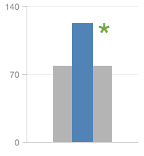
We can use a bullet chart and a headline report to depict hypothesis testing as shown below:

The bullet shows the sample mean, and the bar shows the population mean. Using conditional formatting on the p-value metric, we can create an asterisk headline report to depict the significance.

Hypothesis Testing – One Sample Z-Tests

Generally speaking, t-distribution tests are used for small sample analyses where fewer than 150 observations are available. Mathematically, the t-distribution becomes more similar to the normal distribution with each additional observation.

For more than 30 observations, they are extremely similar, and for more than 100, you would be unlikely to notice the difference between the normal distribution and t-distribution. When more than 150 observations are available, we should use the z-distribution (a.k.a. normal distribution).

For this reason, we have designed the MAQL metrics (df for p-value) and the underlying table to automatically switch from the t-distribution to the normal distribution when there are more than 150 observations. So, you don’t need to distinguish the t-test and z-test when using this methodology.

The same example table can be used to perform F-tests/ANOVAs, Chi-squared Goodness of Fit tests, and other t-tests/z-tests.