How to Use MAQL Count in GoodData.CN
Version Compatibility Notice
The content of this article is valid for the version of GoodData that was current as of 3 August 2021. Features or behavior in newer versions may differ.
Count is one of the most used aggregation functions. However, it is a MAQL function commonly misunderstood as the same Count function used in SQL. In this article, we will explore the MAQL function and understand how to use this function in GoodData.CN.
The count function is an aggregation function that counts the distinct value of the selected attribute. In GoodData.CN, the count function has a different syntax to accommodate different LDM designs. Count can be used in the following syntax as mentioned in the documentation:
Count(attribute), Count(attribute, primary_key), Count(attribute) using primary_key
In his article, we will explore how we can use Count(attribute), Count(attribute, primary_key) for different designs of LDM, purposes, and situations. We will start with the first example to explain how to use Count(attribute):
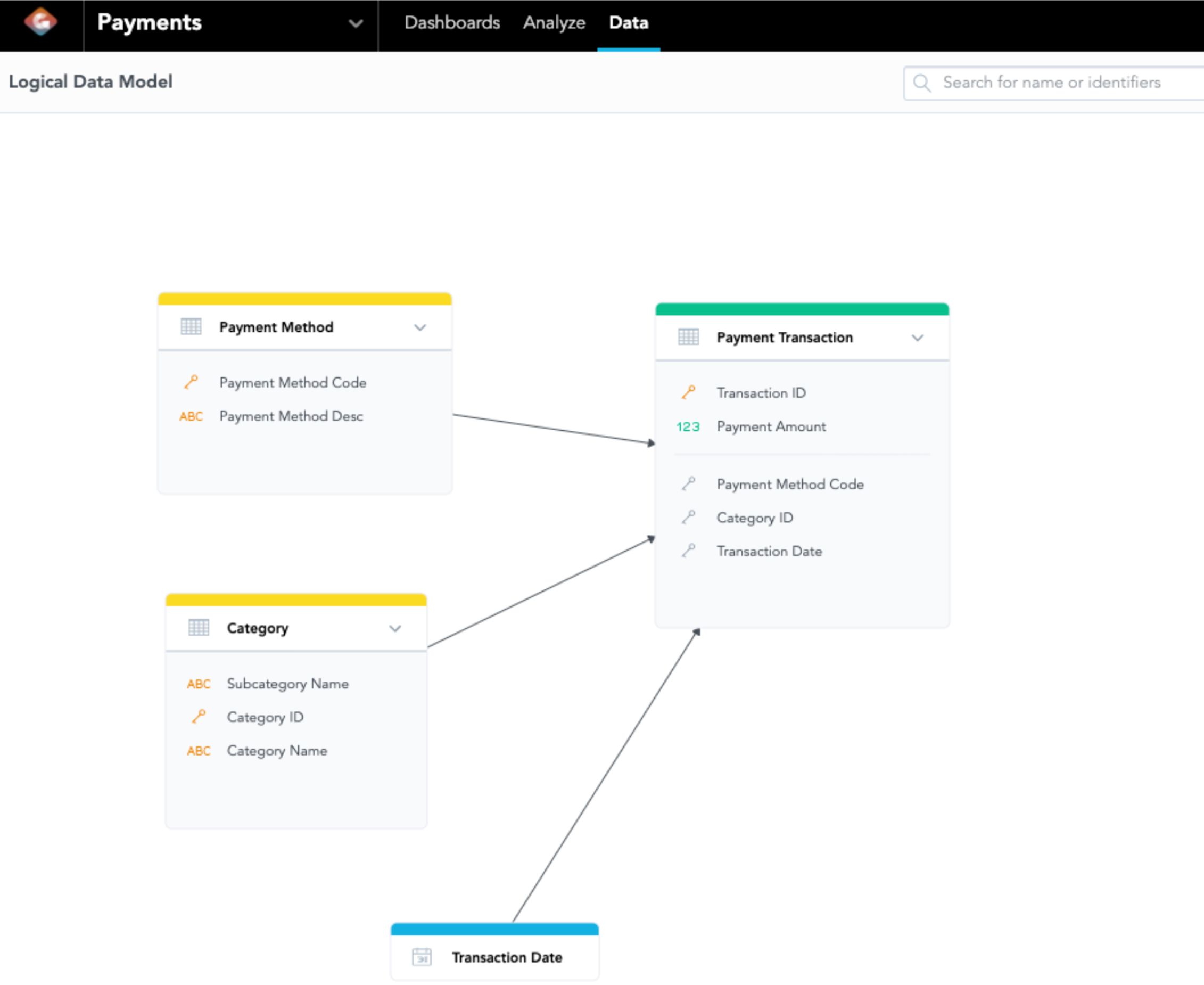
We have a small sales data set of a hypothetical small retail company; the data set consists of details of transactions. Before building the MAQL query, we shall first look at the Logical Data Model (LDM) to understand the relationship among the attributes and facts in the data set. Below is Diagram 1, which shows the LDM and its metadata of this hypothetical small retail company.
| Type | ID | Column Name |
|---|---|---|
| Attribute | paymentmethod.paymentmethodcode | Payment Method Code |
| Attribute | paymentmethod.paymentmethoddesc | Payment Method Desc |
| Attribute | category.categoryid | Category ID |
| Attribute | category.categoryname | Category Name |
| Attribute | category.subcategory | Subcategory Name |
| Attribute | paymenttransaction.transactionid | Transaction ID |
| Fact | paymenttransaction.paymentamount | Payment Amount |
| Date | transactiondate.<Date Granularity> | Transaction Date |
Table 1: LDM Metadata of the Workspace
The LDM tells you the relationship between attributes and facts about the data sets while the metadata is automatically generated by GoodData.CN for users to define new metrics. In GoodData.CN, you will use the column ID to build any MAQL query, so verifying the LDM metadata is very important. The count function highly depends on this model; it is very useful when you are trying to find a primary key when using count(attribute, primary_key) later.
We are interested in finding out how many different types of payments there are during check-outs. Therefore, we can use MAQL to build a count function to answer our question. We know that the column ID of the payment method code is paymentmethod.paymethodcode from Table 1, and we can simply put in the custom metric page:
SELECT COUNT({attribute/paymentmethod.paymentmethodcode}) - Syntax 1
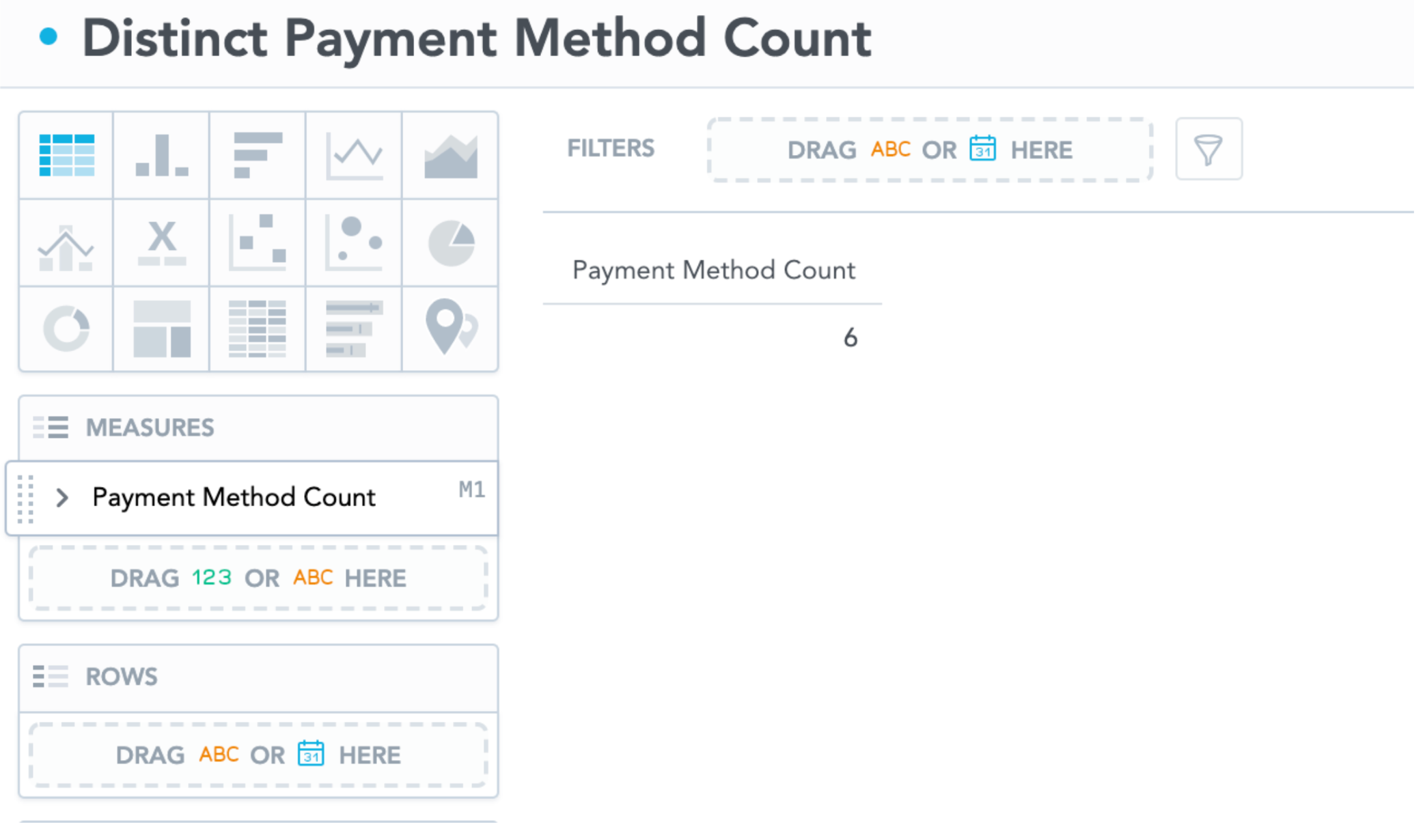
The syntax allows GoodData.CN to count distinct values of Payment Method Code among the transactions in the data set. We may get this result:
Diagram 2: Table of Distinct Payment Method Count
If we apply Syntax 1 when creating this table in the analytical designer, it tells GoodData.CN to count the number of distinct values of the payment method at the current level, which is the whole data set in our case. It tells you there are 6 payment methods that appear in the data set, but it is not the same idea as the number of distinct payment methods in all transactions. From a business perspective, we may be more interested in looking at how many payment methods are used in all transactions. If this is the case, Syntax 1 may not work the way we intended because we want the GoodData.CN to count payment methods on the transaction data level. In order to tell GoodData.CN what context to look at, we need to pass a primary key in Count(attribute, primary_key). The primary key is a connection point between data sets; it tells the context of the data to count from. Before doing this, we need to check whether it is valid to do so from the LDM.
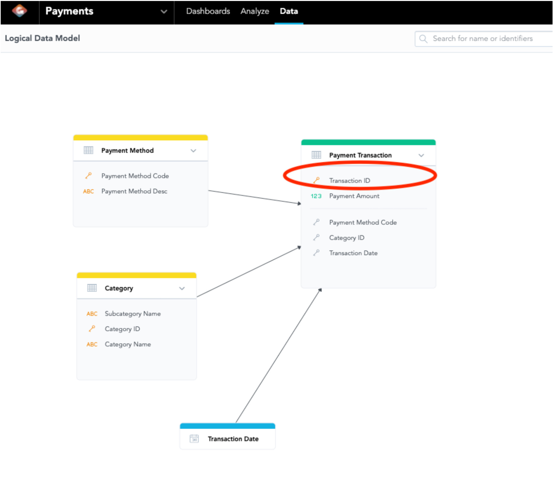
Diagram 3: Looking for Central Data Set in the LDM
Now, the question is, what should I pick as the primary key to use in the Count() function? First, find the data set referenced from the data set containing the attribute you are counting (The data set has a lot of edges pointing at it). Then, pick the primary key in the data set that is being referenced. If we look at Diagram 2, we can see the data set Payment Method points at the data set Payment Transaction. The Transaction ID is the primary key of Payment Transaction so we will pick Transaction ID as the primary key in the Count() function. And therefore, we create Syntax 2 below:
SELECT COUNT({attribute/paymentmethod.paymentmethodcode},{attribute/paymenttransaction.transactionid}) - Syntax 2
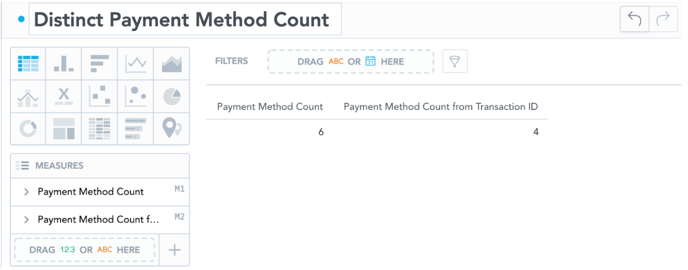
If we declare a metric using syntax 2 (And call it Payment Method Count from Transaction ID), GoodData.CN would now be able to find the number of distinct payment methods used in all transactions.
Diagram 4: Difference Between not using the primary key (Left) and using the primary key (Right)
As we can see in Diagram 4, it makes a difference between using and not using the primary key as it informs GoodData.CN how to look at the data. We have 6 payment methods in the data set; only 4 payment methods were used among all transactions. The left column shows that there are 6 available payment method types to customers; the right column shows customers have used only 4 payment method types to pay. It means we have found that no customer has ever used two of the payment methods during check-outs.
LDM is also useful to know what attributes can be sliced from one attribute because a metric or fact can only be sliced by related attributes. If we look at Diagram 3 again, we know that Count(Payment Method type, Transaction ID) can be segmented by Category ID, Payment Method Type, and Transaction Date because the datasets they belong to reference the Payment Transaction dataset (They both have edges pointing at Transaction ID). We called Payment Transaction a central dataset as it has many attributes referencing, while the primary key of Payment Transaction dataset is the central attribute; in our case, that would be Transaction ID. Most of the time, the central attribute is the best primary key to use.
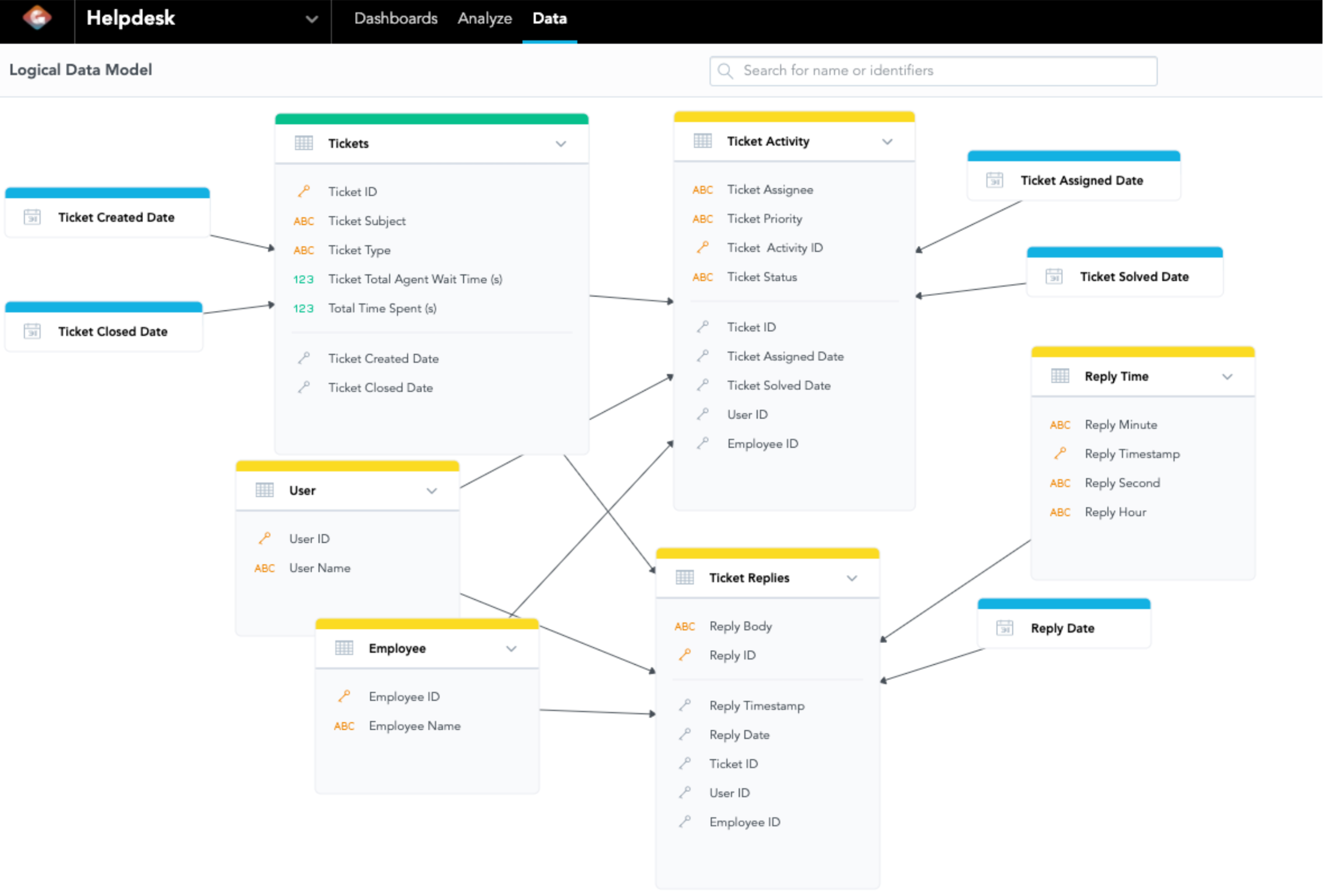
When the LDM is complex, a primary key used in the count function becomes critical because it determines what attributes can be sliced by. There is a limitation to the MAQL count function: The metric is only allowed to be sliced by the attributes connected to what you are counting on. In the following example, consider we have a help desk, and we would like to understand how many employees are involved in each ticket. It has an LDM and the metadata of selected columns in the LDM below:
Diagram 5: LDM of a Help Desk Data Set
| Type | ID | Table Name | Column Name |
|---|---|---|---|
| Attribute | ticketreplies.replyid | Ticket Replies | Reply ID |
| Attribute | ticketreplies.replybody | Ticket Replies | Reply Body |
| Attribute | employees.employeesid | Employees | Employee ID |
| Attribute | user.userid | User | User ID |
| Attribute | tickets.ticketid | Tickets | Ticket ID |
| Attribute | replytime.replytimestamp | Reply Time | Reply Timestamp |
| Date | replydate.<Date Granularity> | Reply Date | Reply Date |
Table 2: Metadata of the Selected Columns in the Help Desk Data Set
Table 2: Metadata of the Selected Columns in the Help Desk Data Set
Now, our goal is to find how many employees reply to each ticket. In this LDM, we can find 2 central datasets - Ticket Activity and Ticket Replies. We can tell those datasets are central datasets because they both have plenty of attributes or facts referencing. If you look at the LDM in Diagram 5, we can trace the data set where the Employee ID belongs. Employee is pointing to Ticket Replies, which also has a lot of edges pointing to. Since Ticket Replies have many edges pointing to it, it is a good primary key to use in our count function to use Reply ID.
SELECT COUNT({attribute/employees.employeeid},{attribute/ticketreplies.replyid}) - Syntax 3


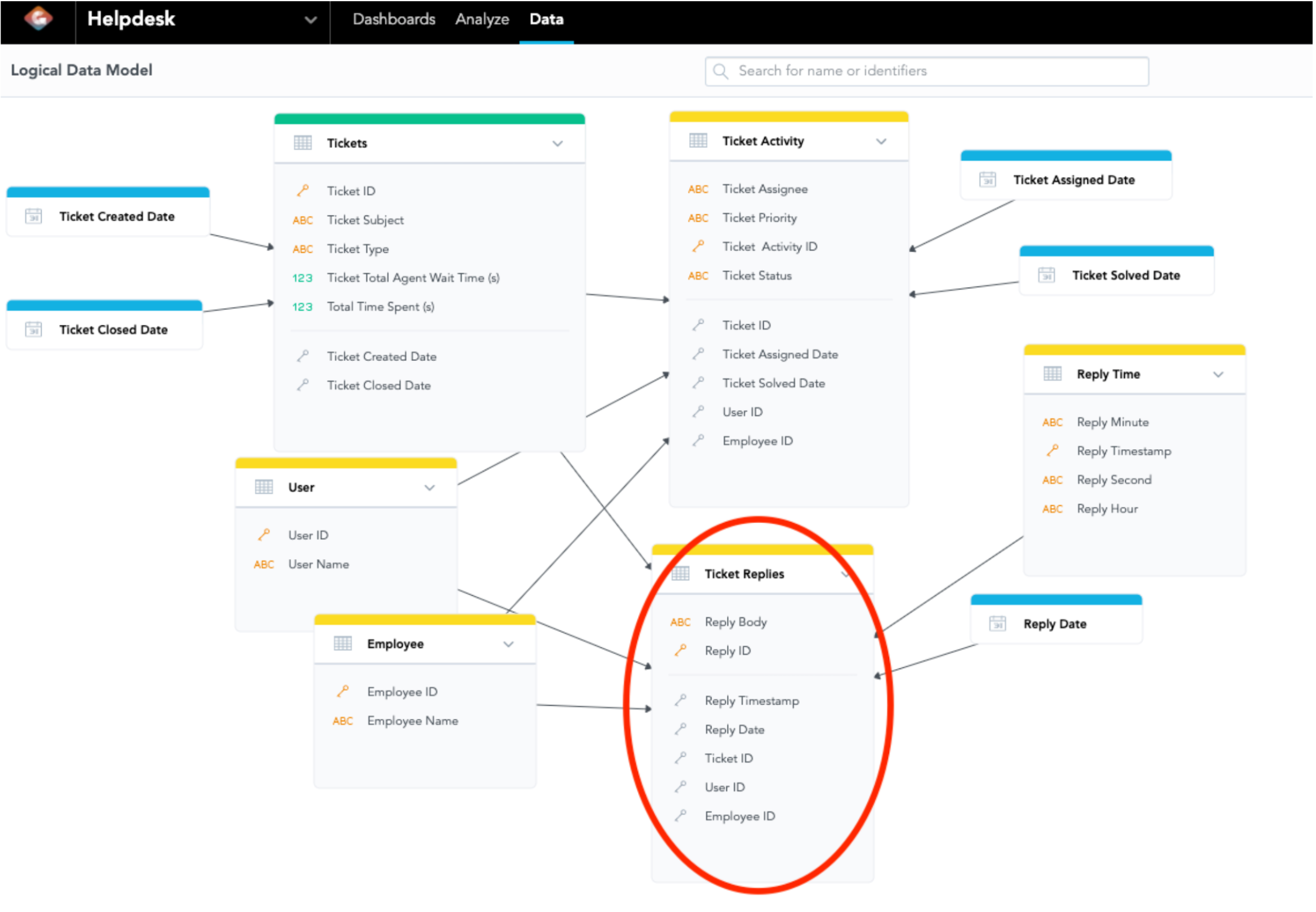
**Diagram 6: LDM of a Call Center Data Set, Attributes connected to Records of Ticket Replies**

As we have discussed, you can see what Syntax 3 can be sliced by legally in the LDM. If we look at the LDM, we can see the following attributes in the data set Ticket Replies (Circled in red in Diagram 8):

1. Reply ID
2. Reply Body
3. Ticket ID
4. User ID
5. Reply Timestamp
6. Reply Date

While we define Syntax 3, we can slice the metric by the above attributes without a problem.

You may discover the limitation that you are not able to slice by any attribute with the data set that has no edge pointing at Ticket Replies. Let’s say you use the metric of Syntax 3 and try to slice by Ticket Priority in the Ticket Activity dataset. Once you have selected this metric on insight, GoodData.CN will update the available attributes on the left panel in the analytical designer, "Ticket Priority" was taken away (So do Ticket Assignee, Ticket Status, Assigned Date, and Solved Date). Since Ticket Priority does not have a direct relationship with the Ticket Replies dataset, it is not possible to slice Ticket Priority from the metric of Syntax 3. Therefore, it is wise to think ahead on designing metrics while designing the LDM.

The best practice for using the Count function is to first know what metrics you would like to have and design an LDM based on that. Then, look at the attribute you would like to count, observe what other attribute it points at, or look for a central dataset in the LDM. Define the Count function by including an attribute and a primary key, especially if there is more than 1 central dataset.

The MAQL Count function is a powerful function that helps you to count the number of distinct values of an attribute while slicing by other related attributes. Before defining the metric using the Count function, the very first thing you need to do is understand the LDM and observe the relationship between the attribute you want to count and other attributes. Then, you can slice the metric by any attribute related to the attributes you are counting.

---

### If you are interested in GoodData.CN, please contact us.

Alternatively, test the trial version of GoodData Cloud: [Start Your GoodData Analytics Trial — Commitment-Free](https://www.gooddata.com/trial/)
