Reading the Model

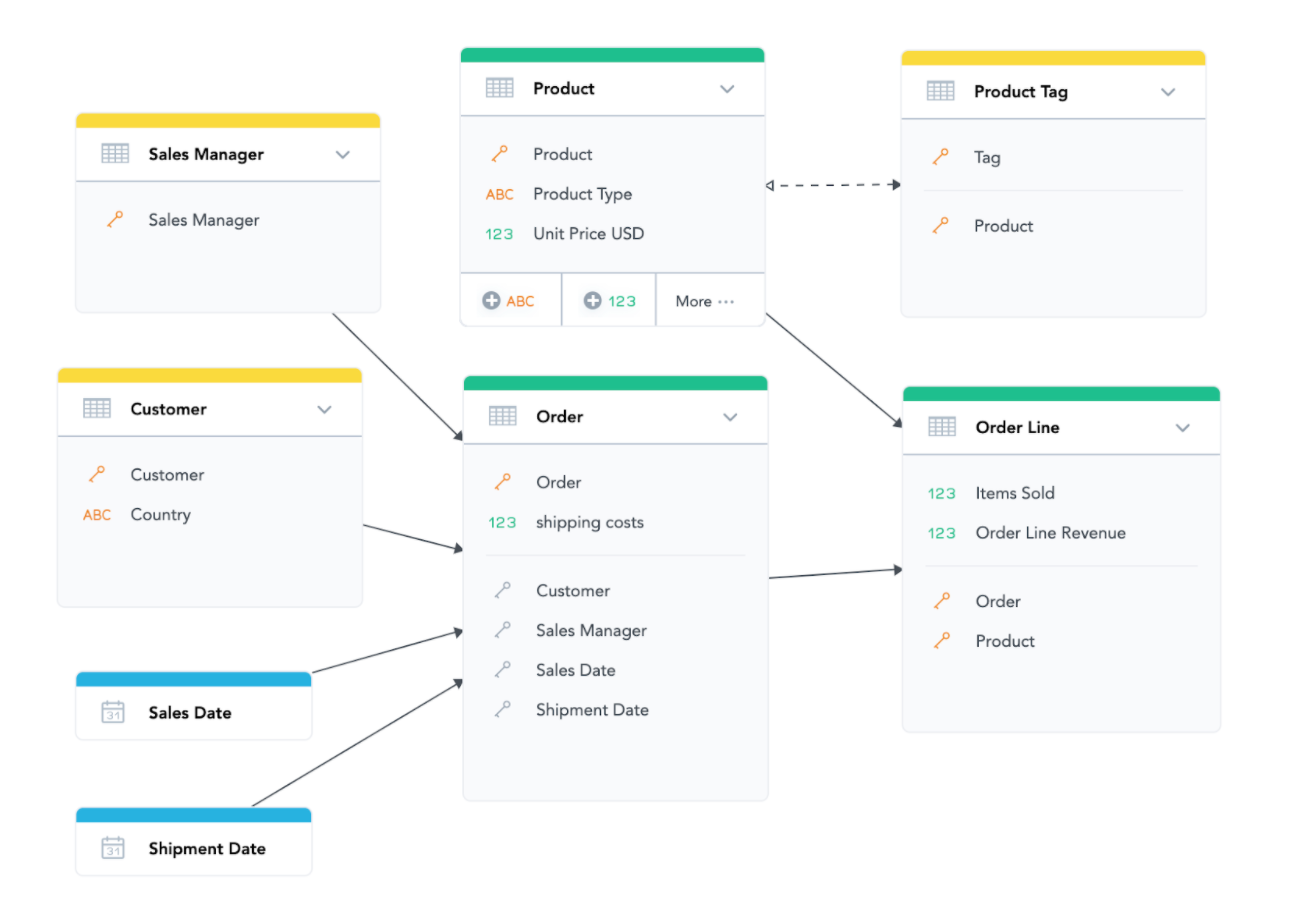
To use and possibly design logical data models, you need to understand how to read them. They tell you a lot, most importantly how the data is structured in a workspace but also which types of insights and measures you can and cannot create with them. It sounds a bit complicated, but it is actually quite simple. Let’s again take a look at our sample logical data model for Acme: 

There are a few basic rules about which parts can interact with each other.

Within a single dataset, slicing and filtering is possible

That is expected and unsurprising. You can, for example, filter customers by country, or you can calculate the “average unit price” (which would be a measure based on the “Unit Price USD” fact that exists in the Product dataset) by Product Type (which also exists in the Product dataset).

Across different datasets, the arrows (relationships) and their direction matter

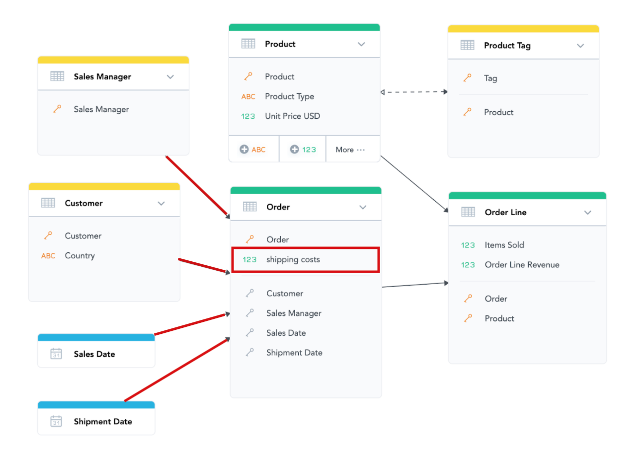
Once the analysis crosses the border of a single dataset, we need to follow the arrows. Measures based on “Shipping Costs” (in the Order dataset) can be filtered by the Order attribute (the ID of the order) based on the previous rule, but it can also be filtered by any attribute from the “Customer” and “Sales Manager” datasets. That is because there is a one-to-many relationship defined between “Order” and the other datasets. We can get to the Order dataset from the other datasets if we follow the direction of the arrows. We can use any attribute from datasets that point to the Orders dataset to slice and filter “Shipping Costs” based measures with. This also works for dates, so “Shipping Costs” based measures can also be filtered and sliced by attributes from both of the date dimensions.

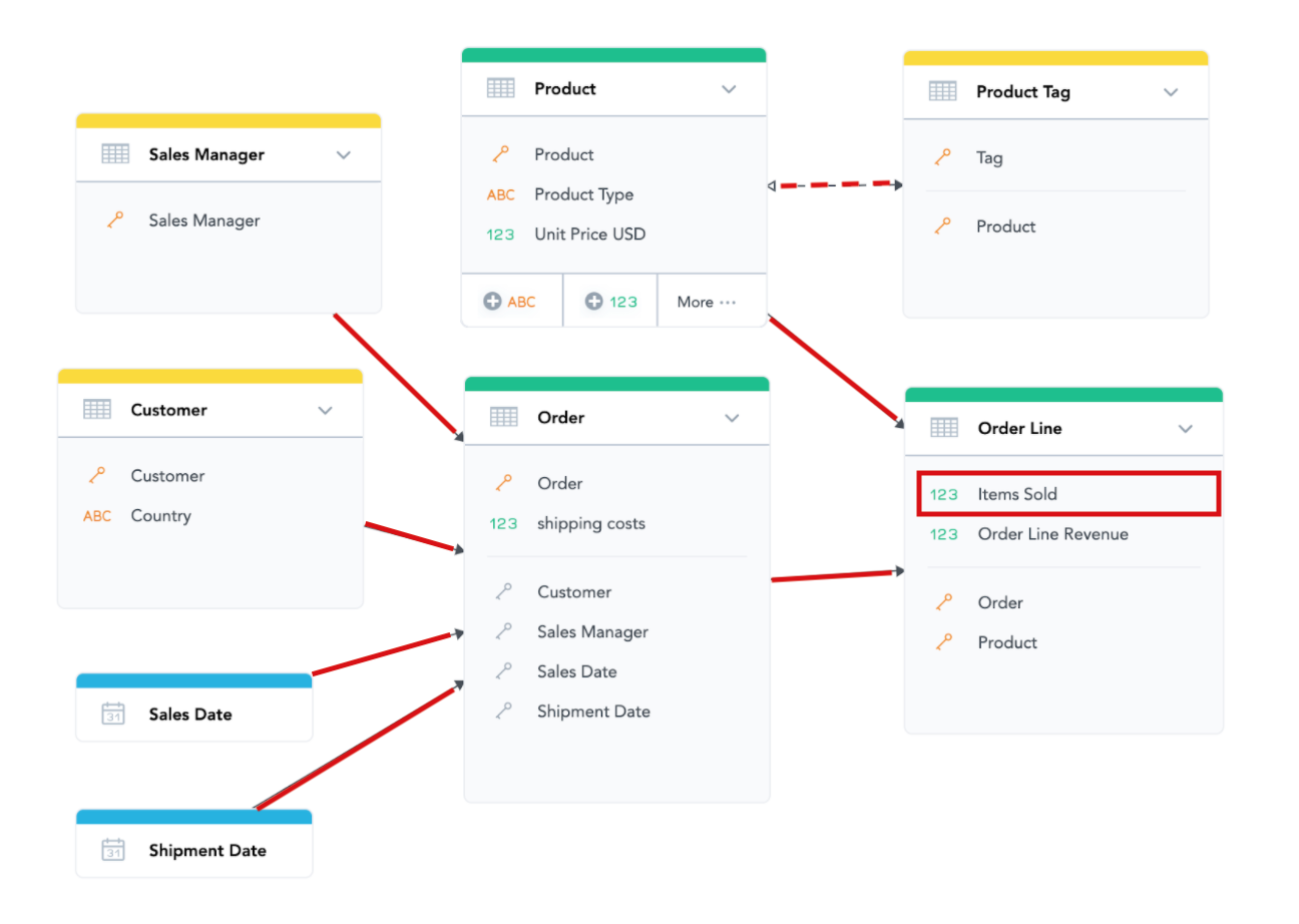
This even works across multiple datasets. Measures based on the “Items Sold” fact (residing in the “Order Line” dataset) can also be sliced and filtered by any attribute in the “Customer” and “Sales Manager” datasets because there is an oriented path going from those datasets to the “Order Line” dataset.

For the many-to-many relationship, this rule works in a similar way; you can treat the double-sided arrow as if it goes in any direction, so “Items Sold” can be filtered and sliced by “Tag.”

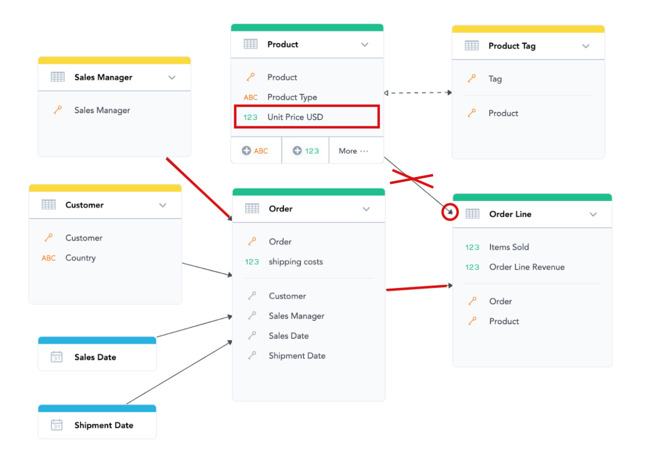
On the other hand, measures based on “Unit Price USD” (from the Product dataset) cannot be filtered or sliced by Sales Manager, because we cannot get from the Sales Manager dataset to the Product dataset following the direction of the arrows (specifically because of the direction of the arrow from Product to Order Lines).

It might look complicated at first sight, but it makes a lot of sense; the unit price here represents the current selling price of that particular product and is only related to the product itself, not to any specific order. The price for which the product was sold in each order is actually in the “Order Line” dataset as another fact called “Order Line Revenue.” This one (because it is in the “Order Line” dataset) can be aggregated and filtered by any of the attributes and dates in the model, because there is an oriented path from all the other datasets to the Order Line dataset. Additionally, the platform automatically hides the incompatible attributes, facts, and measures from the catalog when you are building insights in the Analytical Designer.

To sum the rules up: “You can slice and filter by anything from the same dataset or from datasets from which an oriented path to your dataset exists.”

You might have noticed that we say a “measure based on a fact can/cannot be filtered/sliced” instead of just “a fact can be sliced.” When analyzing data in GoodData, you always aggregate it in some way—i.e., a sum of Items Sold or average unit price—the resulting calculation is called a measure. The measures can then be used in the Analytical Designer to create insights. Measures can be much more complicated than just a simple sum or average.

Coming up next is a short quiz that will allow you to practice what you just learned!